MadMiner physics tutorial (part 4C)

Johann Brehmer, Felix Kling, Irina Espejo, and Kyle Cranmer 2018-2019

0. Preparations

import logging
import numpy as np
import matplotlib
from matplotlib import pyplot as plt
%matplotlib inline

from madminer.fisherinformation import FisherInformation, InformationGeometry
from madminer.plotting import plot_fisher_information_contours_2d

# MadMiner output
logging.basicConfig(
    format='%(asctime)-5.5s %(name)-20.20s %(levelname)-7.7s %(message)s',
    datefmt='%H:%M',
    level=logging.INFO
)

# Output of all other modules (e.g. matplotlib)
for key in logging.Logger.manager.loggerDict:
    if "madminer" not in key:
        logging.getLogger(key).setLevel(logging.WARNING)

Let’s look at a simple example to understand what happens in information geometry. At first we note that the Fisher Information is a symmetric positive definite rank two tensor, and therefore can be seen as a Riemanian metric. It can therefore be used to calculate distances between points in parameter space.

Previously, in tutorial 4b, we have considered the local distance \(d_{local}(\theta,\theta_0)\) between two points \(\theta\) and \(\theta_0\). It is defined in the tangent space of \(\theta_0\), where the metric is constant and hence flat, and can simply be calculated as \(d_{local}(\theta,\theta_0) = I_{ij}(\theta_0) \times (\theta-\theta_0)^i (\theta-\theta_0)^j\).

Going beyond this local approximation, we can calculate a global distance \(d_{global}(\theta,\theta_0)\) which takes into account the fact that the information is not constant throughout the parameter space. Using our knowledge from general relativity, this distance is defined as

\[ d(\theta,\theta_0)= \text{min} \int_{\theta_0}^{\theta} ds \sqrt{I_{ij}(\theta(s)) \frac{d\theta^i}{ds}\frac{d\theta^j}{ds}} \]

where \(\theta(s)\) is the geodesic (the shortest path) connecting \(\theta_0\) and \(\theta\). This path follows the geodesic equation

\[ \frac{d^2\theta^i}{ds^2} = - \Gamma^i_{jk} \frac{d\theta^j}{ds}\frac{d\theta^k}{ds} \quad \text{with} \quad \Gamma^i_{jk} = \frac{1}{2} I^{im} \Big(\frac{\partial I_{mk}}{\partial \theta^j} + \frac{\partial I_{mj}}{\partial \theta^k} - \frac{\partial I_{jk}}{\partial \theta^m}\Big) \quad \text{and} \quad I^{im} I_{mj} = \delta^i_j \]

In practice, we obtain the geodesics by numerically integrating the geodesic equation, starting at a parameter point \(\theta_0\) with a velocity \(\theta'_0=(\frac{\theta}{ds})_0\).

1. Stand Alone Example

In this example we consider a sample geometry with Fisher Information \(I_{ij}(\theta)= (( 1 + \frac{\theta_1}{4}, 1 ), ( 1, 2 - \frac{\theta_2}{2}))\) and determine the geodesics and distance contours for illustration. At first, we initialize a new instance of class InformationGeometry and define the Fisher Information via the function information_from_formula().

formula="np.array([[1 + 0.25*theta[0] ,1],[1, 2 - 0.5*theta[1]  ]])"

infogeo=InformationGeometry()
infogeo.information_from_formula(formula=formula,dimension=2)

Now we obtain one particular geodesic path staring at \(\theta_0\) in the direction of \(\Delta \theta_0\) using the function find_trajectory().

thetas,distances=infogeo.find_trajectory(
    theta0=np.array([0.,0.]),
    dtheta0=np.array([1.,1.]),
    limits=np.array([[-1.,1.],[-1.,1.]]),
    stepsize=0.025,
)

For comparisson, let’s do the same for a constant Fisher Information \(I_{ij}(\theta)=I_{ij}(\theta_0)=((1,1),(1,2))\).

formula_lin="np.array([[1 ,1],[1, 2 ]])"
infogeo_lin=InformationGeometry()
infogeo_lin.information_from_formula(formula=formula_lin,dimension=2)
thetas_lin,distances_lin=infogeo_lin.find_trajectory(
    theta0=np.array([0.,0.]),
    dtheta0=np.array([1.,1.]),
    limits=np.array([[-1.,1.],[-1.,1.]]),
    stepsize=0.025,
)

and plot the results

cmin, cmax = 0., 2
fig = plt.figure(figsize=(6,5))

plt.scatter(
    thetas_lin.T[0],thetas_lin.T[1],c=distances_lin,
    s=10., cmap='viridis',marker='o',vmin=cmin, vmax=cmax,
)
sc = plt.scatter(
    thetas.T[0],thetas.T[1],c=distances,
    s=10., cmap='viridis',marker='o',vmin=cmin, vmax=cmax,
)
plt.scatter( [0],[0],c='k')

cb = plt.colorbar(sc)
cb.set_label(r'Distance $d(\theta,\theta_0)$')

plt.xlabel(r'$\theta_1$')
plt.ylabel(r'$\theta_2$')
plt.tight_layout()
plt.show()

We can see that the geodesic trajectory is curved. The colorbar denotes the distance from the origin.

Let us now see how we can construct the distance contours using the function distance_contours.

grid_ranges = [(-1, 1.), (-1, 1.)]
grid_resolutions = [25, 25]

theta_grid,p_values,distance_grid,(thetas,distances)=infogeo.distance_contours(
    np.array([0.,0.]),
    grid_ranges=grid_ranges, 
    grid_resolutions=grid_resolutions,
    stepsize=0.08,
    ntrajectories=30,
    continous_sampling=True,
    return_trajectories=True,   
)

and plot the results

#Prepare Plot
cmin, cmax = 0., 2
fig = plt.figure(figsize=(15.0, 4.0 ))

bin_size = (grid_ranges[0][1] - grid_ranges[0][0])/(grid_resolutions[0] - 1)
edges = np.linspace(grid_ranges[0][0] - bin_size/2, grid_ranges[0][1] + bin_size/2, grid_resolutions[0] + 1)
centers = np.linspace(grid_ranges[0][0], grid_ranges[0][1], grid_resolutions[0])

#Plot
ax = plt.subplot(1,3,1)
sc = ax.scatter(thetas.T[0],thetas.T[1],c=distances,vmin=cmin, vmax=cmax,)
cb = plt.colorbar(sc,ax=ax, extend='both')
cb.set_label(r'Distance $d(\theta,\theta_0)$')
ax.set_xlabel(r'$\theta_1$')
ax.set_ylabel(r'$\theta_2$')


ax = plt.subplot(1,3,2)
cm = ax.pcolormesh(
    edges, edges, distance_grid.reshape((grid_resolutions[0], grid_resolutions[1])).T,
    vmin=cmin, vmax=cmax,
    cmap='viridis'
)
cb = plt.colorbar(cm, ax=ax, extend='both')
cb.set_label(r'Distance $d(\theta,\theta_0)$')
ax.set_xlabel(r'$\theta_1$')
ax.set_ylabel(r'$\theta_2$')


ax = plt.subplot(1,3,3)
cm = ax.pcolormesh(
    edges, edges, p_values.reshape((grid_resolutions[0], grid_resolutions[1])).T,
    norm=matplotlib.colors.LogNorm(vmin=0.1, vmax=1),
    cmap='viridis'
)
cb = plt.colorbar(cm, ax=ax, extend='both')
cb.set_label('Expected p-value')
ax.set_xlabel(r'$\theta_1$')
ax.set_ylabel(r'$\theta_2$')


plt.tight_layout()
plt.show()

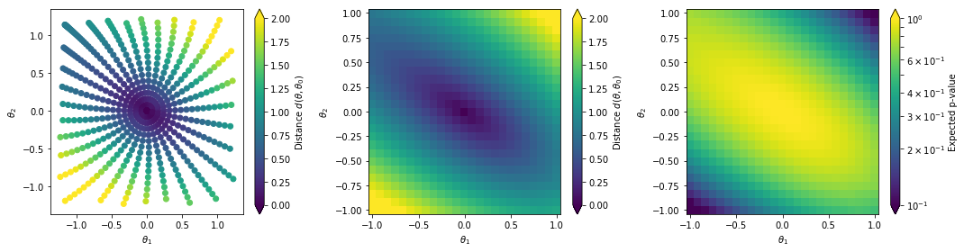
The left plot shows the distance values along generated geodesics. These values are interpolated into a continuous function shown in the middle plot. In the right plot we convert the distances into expected p-values.

2. Information Geometry Bounds for Example Process

Now that we understand how Information Geometry works in principle, let’s apply it to our example process. Let’s first create a grid of theta values

def make_theta_grid(theta_ranges, resolutions):
        theta_each = []
        for resolution, (theta_min, theta_max) in zip(resolutions, theta_ranges):
            theta_each.append(np.linspace(theta_min, theta_max, resolution))
        theta_grid_each = np.meshgrid(*theta_each, indexing="ij")
        theta_grid_each = [theta.flatten() for theta in theta_grid_each]
        theta_grid = np.vstack(theta_grid_each).T
        return theta_grid
    
grid_ranges = [(-1, 1.), (-1, 1.)]
grid_resolutions = [25, 25]
theta_grid = make_theta_grid(grid_ranges,grid_resolutions)

Now we create a grid of Fisher Informations. Since this might take some time, we already prepared the results, which can be loaded directly.

model='alices'
calculate_fisher_grid=False
if calculate_fisher_grid:
    fisher = FisherInformation('data/lhe_data_shuffled.h5')
    fisher_grid=[]

    for theta in theta_grid:
        fisher_info, _ = fisher.full_information(
            theta=theta,
            model_file='models/'+model,
            luminosity=300.*1000.,
            include_xsec_info=False,
        )
        fisher_grid.append(fisher_info)
    np.save(f"limits/infogeo_thetagrid_{model}.npy", theta_grid)
    np.save(f"limits/infogeo_fishergrid_{model}.npy", fisher_grid)
else: 
    theta_grid=np.load(f"limits/infogeo_thetagrid_{model}.npy")
    fisher_grid=np.load(f"limits/infogeo_fishergrid_{model}.npy")

In the next step, we initialize the InformationGeometry class using this input data. Using the function information_from_grid(), the provided grid is interpolated using a piecewise linear function and the information can be calculated at every point.

infogeo=InformationGeometry()
infogeo.information_from_grid(
    theta_grid=f"limits/infogeo_thetagrid_{model}.npy",
    fisherinformation_grid=f"limits/infogeo_fishergrid_{model}.npy",
)

14:05 madminer.utils.vario INFO      Loading limits/infogeo_thetagrid_alices.npy into RAM
14:05 madminer.utils.vario INFO      Loading limits/infogeo_fishergrid_alices.npy into RAM

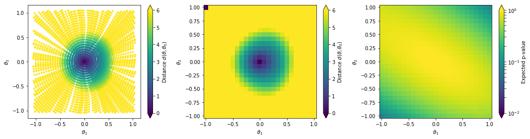
As before, we can now obtain the p-values using the distance_contours() function

theta_grid,p_values_infogeo,distance_grid,(thetas,distances)=infogeo.distance_contours(
    np.array([0.,0.]),
    grid_ranges=grid_ranges, 
    grid_resolutions=grid_resolutions,
    stepsize=0.05,
    ntrajectories=300,
    return_trajectories=True,   
)

and plot it again

#Prepare Plot
cmin, cmax = 0., 6
fig = plt.figure(figsize=(15.0, 4.0 ))

bin_size = (grid_ranges[0][1] - grid_ranges[0][0])/(grid_resolutions[0] - 1)
edges = np.linspace(grid_ranges[0][0] - bin_size/2, grid_ranges[0][1] + bin_size/2, grid_resolutions[0] + 1)
centers = np.linspace(grid_ranges[0][0], grid_ranges[0][1], grid_resolutions[0])

#Plot
ax = plt.subplot(1,3,1)
sc = ax.scatter(thetas.T[0],thetas.T[1],c=distances,vmin=cmin, vmax=cmax,s=10,)
cb = plt.colorbar(sc,ax=ax, extend='both')
cb.set_label(r'Distance $d(\theta,\theta_0)$')
ax.set_xlabel(r'$\theta_1$')
ax.set_ylabel(r'$\theta_2$')


ax = plt.subplot(1,3,2)
cm = ax.pcolormesh(
    edges, edges, distance_grid.reshape((grid_resolutions[0], grid_resolutions[1])).T,
    vmin=cmin, vmax=cmax,
    cmap='viridis'
)
cb = plt.colorbar(cm, ax=ax, extend='both')
cb.set_label(r'Distance $d(\theta,\theta_0)$')
ax.set_xlabel(r'$\theta_1$')
ax.set_ylabel(r'$\theta_2$')


ax = plt.subplot(1,3,3)
cm = ax.pcolormesh(
    edges, edges, p_values.reshape((grid_resolutions[0], grid_resolutions[1])).T,
    norm=matplotlib.colors.LogNorm(vmin=0.01, vmax=1),
    cmap='viridis'
)
cb = plt.colorbar(cm, ax=ax, extend='both')
cb.set_label('Expected p-value')
ax.set_xlabel(r'$\theta_1$')
ax.set_ylabel(r'$\theta_2$')


plt.tight_layout()
plt.show()

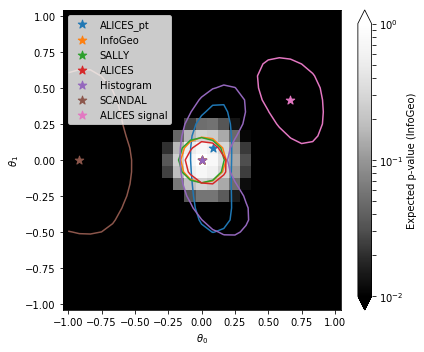
3. Compare to other results

Load previous results and add Information Geometry results

[p_values,mle]=np.load("limits/limits.npy", allow_pickle=True)

p_values["InfoGeo"] = p_values_infogeo.flatten()
mle["InfoGeo"] = 312

and plot them together with the obtained Information Geometry results

show = "InfoGeo"

bin_size = (grid_ranges[0][1] - grid_ranges[0][0])/(grid_resolutions[0] - 1)
edges = np.linspace(grid_ranges[0][0] - bin_size/2, grid_ranges[0][1] + bin_size/2, grid_resolutions[0] + 1)
centers = np.linspace(grid_ranges[0][0], grid_ranges[0][1], grid_resolutions[0])

fig = plt.figure(figsize=(6,5))
ax = plt.gca()

cmin, cmax = 1.e-2, 1.

pcm = ax.pcolormesh(
    edges, edges, p_values[show].reshape((grid_resolutions[0], grid_resolutions[1])).T,
    norm=matplotlib.colors.LogNorm(vmin=cmin, vmax=cmax),
    cmap='Greys_r'
)
cbar = fig.colorbar(pcm, ax=ax, extend='both')

for i, (label, p_value) in enumerate(p_values.items()):
    plt.contour(
        centers, centers, p_value.reshape((grid_resolutions[0], grid_resolutions[1])).T,
        levels=[0.32],
        linestyles='-', colors='C{}'.format(i)
    )
    plt.scatter(
        theta_grid[mle[label]][0], theta_grid[mle[label]][1],
        s=80., color='C{}'.format(i), marker='*',
        label=label
    )

plt.legend()

plt.xlabel(r'$\theta_0$')
plt.ylabel(r'$\theta_1$')
cbar.set_label('Expected p-value ({})'.format(show))

plt.tight_layout()
plt.show()

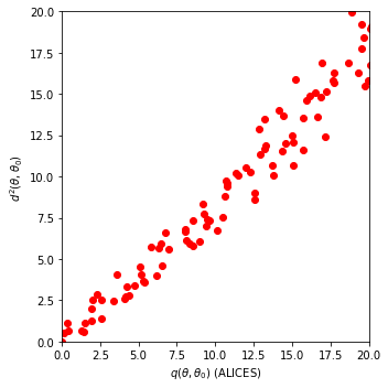
Finally, we compare the obtained distance \(d(\theta,\theta_0)\) with the expected log-likelihood ratio \(q(\theta,\theta_0) = E[-2 \log r(x|\theta,\theta_0)|\theta_0]\). We can see that there is an approximately linear relationship.

from scipy.stats.distributions import chi2

#Prepare Plot
cmin, cmax = 0., 6
fig = plt.figure(figsize=(5.0, 5.0 ))

#Plot
ax = plt.subplot(1,1,1)
ax.scatter(chi2.ppf(1-p_values["ALICES"], df=2),distance_grid.flatten()**2,c="red",)
ax.set_xlabel(r'$q(\theta,\theta_0)$ (ALICES)')
ax.set_ylabel(r'$d^2(\theta,\theta_0)$ ')
ax.set_xlim(0,20)
ax.set_ylim(0,20)

plt.tight_layout()
plt.show()