Appendix 2: Ensemble methods#
Johann Brehmer, Felix Kling, Irina Espejo, and Kyle Cranmer 2018-2019
Instead of using a single neural network to estimate the likelihood ratio, score, or Fisher information, we can use an ensemble of such estimators. That provides us with a more reliable mean prediction as well as a measure of the uncertainty. The class madminer.ml.EnsembleForge automates this process. Currently, it only supports SALLY estimators:
estimators = [ScoreEstimator(n_hidden=(20,)) for _ in range(5)]

ensemble = Ensemble(estimators)
Training#
The EnsembleForge object has very similar functions as MLForge. In particular, we can train all estimators simultaneously with train_all() and save the ensemble to files:
ensemble.train_all(
    method='sally',
    x='data/samples/x_train.npy',
    t_xz='data/samples/t_xz_train.npy',
    n_epochs=5,
)

ensemble.save('models/sally_ensemble')
Evaluation#
We can evaluate the ensemble similarly to the individual networks. Let’s stick to the estimation of the Fisher information. There are two different ways to take the ensemble average:
mode='information': We can calculate the Fisher information for each estimator in the ensemble, and then take the mean and the covariance over the ensemble. This has the advantage that it provides a direct measure of the uncertainty of the prediction.mode='score': We can calculate the score for each event and estimator, take the ensemble mean for the score of each event, and then calculate the Fisher information based on the mean scores. This is expected to be more precise (since the score estimates will be more precise, and the nonlinearity in the Fisher info calculation amplifies any error in the score estimation). But calculating the covariance in this approach is computationally not feasible, so there will be no error bands.
By default, MadMiner uses the ‘score’ mode. Here we will use the ‘information’ mode just to show the nice uncertainty bands we get.
fisher = FisherInformation('data/madminer_example_shuffled.h5')

fisher_information_mean, fisher_information_covariance = fisher.calculate_fisher_information_full_detector(
    theta=[0.,0.],
    model_file='models/sally_ensemble',
    luminosity=3000000.,
    mode='information'
)
The covariance can be propagated to the Fisher distance contour plot easily:
_ = plot_fisher_information_contours_2d(
    [fisher_information_mean],
    [fisher_information_covariance],
    xrange=(-1,1),
    yrange=(-1,1)
)

