MadMiner physics tutorial (part 3A)#
Johann Brehmer, Felix Kling, Irina Espejo, and Kyle Cranmer 2018-2019
In part 3A of this tutorial we will finally train a neural network to estimate likelihood ratios. We assume that you have run part 1 and 2A of this tutorial. If, instead of 2A, you have run part 2B, you just have to load a different filename later.
Preparations#
import logging
import numpy as np
import matplotlib
from matplotlib import pyplot as plt
%matplotlib inline

from madminer.sampling import SampleAugmenter
from madminer import sampling
from madminer.ml import ParameterizedRatioEstimator
# MadMiner output
logging.basicConfig(
    format='%(asctime)-5.5s %(name)-20.20s %(levelname)-7.7s %(message)s',
    datefmt='%H:%M',
    level=logging.INFO
)

# Output of all other modules (e.g. matplotlib)
for key in logging.Logger.manager.loggerDict:
    if "madminer" not in key:
        logging.getLogger(key).setLevel(logging.WARNING)
1. Make (unweighted) training and test samples with augmented data#
At this point, we have all the information we need from the simulations. But the data is not quite ready to be used for machine learning. The madminer.sampling class SampleAugmenter will take care of the remaining book-keeping steps before we can train our estimators:
First, it unweights the samples, i.e. for a given parameter vector theta (or a distribution p(theta)) it picks events x such that their distribution follows p(x|theta). The selected samples will all come from the event file we have so far, but their frequency is changed – some events will appear multiple times, some will disappear.
Second, SampleAugmenter calculates all the augmented data (“gold”) that is the key to our new inference methods. Depending on the specific technique, these are the joint likelihood ratio and / or the joint score. It saves all these pieces of information for the selected events in a set of numpy files that can easily be used in any machine learning framework.
sampler = SampleAugmenter('data/lhe_data_shuffled.h5')
# sampler = SampleAugmenter('data/delphes_data_shuffled.h5')
20:34 madminer.analysis    INFO    Loading data from data/lhe_data_shuffled.h5
20:34 madminer.analysis    INFO    Found 2 parameters
20:34 madminer.analysis    INFO    Did not find nuisance parameters
20:34 madminer.analysis    INFO    Found 6 benchmarks, of which 6 physical
20:34 madminer.analysis    INFO    Found 3 observables
20:34 madminer.analysis    INFO    Found 89991 events
20:34 madminer.analysis    INFO      49991 signal events sampled from benchmark sm
20:34 madminer.analysis    INFO      10000 signal events sampled from benchmark w
20:34 madminer.analysis    INFO      10000 signal events sampled from benchmark neg_w
20:34 madminer.analysis    INFO      10000 signal events sampled from benchmark ww
20:34 madminer.analysis    INFO      10000 signal events sampled from benchmark neg_ww
20:34 madminer.analysis    INFO    Found morphing setup with 6 components
20:34 madminer.analysis    INFO    Did not find nuisance morphing setup
The SampleAugmenter class defines five different high-level functions to generate train or test samples:
sample_train_plain(), which only saves observations x, for instance for histograms or ABC;sample_train_local()for methods like SALLY and SALLINO, which will be demonstrated in the second part of the tutorial;sample_train_density()for neural density estimation techniques like MAF or SCANDAL;sample_train_ratio()for techniques like CARL, ROLR, CASCAL, and RASCAL, when only theta0 is parameterized;sample_train_more_ratios()for the same techniques, but with both theta0 and theta1 parameterized;sample_test()for the evaluation of any method.
For the arguments theta, theta0, or theta1, you can (and should!) use the helper functions benchmark(), benchmarks(), morphing_point(), morphing_points(), and random_morphing_points(), all defined in the madminer.sampling module.
Here we’ll train a likelihood ratio estimator with the ALICES method, so we focus on the extract_samples_train_ratio() function. We’ll sample the numerator hypothesis in the likelihood ratio with 1000 points drawn from a Gaussian prior, and fix the denominator hypothesis to the SM.
Note the keyword sample_only_from_closest_benchmark=True, which makes sure that for each parameter point we only use the events that were originally (in MG) generated from the closest benchmark. This reduces the statistical fluctuations in the outcome quite a bit.
x, theta0, theta1, y, r_xz, t_xz, n_effective = sampler.sample_train_ratio(
    theta0=sampling.random_morphing_points(1000, [('gaussian', 0., 0.5), ('gaussian', 0., 0.5)]),
    theta1=sampling.benchmark('sm'),
    n_samples=500000,
    folder='./data/samples',
    filename='train_ratio',
    sample_only_from_closest_benchmark=True,
    return_individual_n_effective=True,
)
20:34 madminer.sampling    INFO    Extracting training sample for ratio-based methods. Numerator hypothesis: 1000 random morphing points, drawn from the following priors:
  theta_0 ~ Gaussian with mean 0.0 and std 0.5
  theta_1 ~ Gaussian with mean 0.0 and std 0.5, denominator hypothesis: sm
20:34 madminer.sampling    INFO    Starting sampling serially
20:34 madminer.sampling    WARNING Large statistical uncertainty on the total cross section when sampling from theta = [-0.35251218 -0.217245  ]: (0.001207 +/- 0.000370) pb (30.639815418386465 %). Skipping these warnings in the future...
20:34 madminer.sampling    INFO    Sampling from parameter point 50 / 1000
20:34 madminer.sampling    INFO    Sampling from parameter point 100 / 1000
20:34 madminer.sampling    INFO    Sampling from parameter point 150 / 1000
20:34 madminer.sampling    INFO    Sampling from parameter point 200 / 1000
20:34 madminer.sampling    INFO    Sampling from parameter point 250 / 1000
20:34 madminer.sampling    INFO    Sampling from parameter point 300 / 1000
20:35 madminer.sampling    INFO    Sampling from parameter point 350 / 1000
20:35 madminer.sampling    INFO    Sampling from parameter point 400 / 1000
20:35 madminer.sampling    INFO    Sampling from parameter point 450 / 1000
20:35 madminer.sampling    INFO    Sampling from parameter point 500 / 1000
20:35 madminer.sampling    INFO    Sampling from parameter point 550 / 1000
20:35 madminer.sampling    INFO    Sampling from parameter point 600 / 1000
20:35 madminer.sampling    INFO    Sampling from parameter point 650 / 1000
20:35 madminer.sampling    INFO    Sampling from parameter point 700 / 1000
20:35 madminer.sampling    INFO    Sampling from parameter point 750 / 1000
20:35 madminer.sampling    INFO    Sampling from parameter point 800 / 1000
20:35 madminer.sampling    INFO    Sampling from parameter point 850 / 1000
20:36 madminer.sampling    INFO    Sampling from parameter point 900 / 1000
20:36 madminer.sampling    INFO    Sampling from parameter point 950 / 1000
20:36 madminer.sampling    INFO    Sampling from parameter point 1000 / 1000
20:36 madminer.sampling    INFO    Effective number of samples: mean 540.594777843479, with individual thetas ranging from 22.802180022668374 to 20938.588332878222
20:36 madminer.sampling    INFO    Starting sampling serially
20:36 madminer.sampling    INFO    Sampling from parameter point 50 / 1000
20:36 madminer.sampling    INFO    Sampling from parameter point 100 / 1000
20:36 madminer.sampling    INFO    Sampling from parameter point 150 / 1000
20:36 madminer.sampling    INFO    Sampling from parameter point 200 / 1000
20:36 madminer.sampling    INFO    Sampling from parameter point 250 / 1000
20:36 madminer.sampling    INFO    Sampling from parameter point 300 / 1000
20:36 madminer.sampling    INFO    Sampling from parameter point 350 / 1000
20:36 madminer.sampling    INFO    Sampling from parameter point 400 / 1000
20:36 madminer.sampling    INFO    Sampling from parameter point 450 / 1000
20:36 madminer.sampling    INFO    Sampling from parameter point 500 / 1000
20:36 madminer.sampling    INFO    Sampling from parameter point 550 / 1000
20:37 madminer.sampling    INFO    Sampling from parameter point 600 / 1000
20:37 madminer.sampling    INFO    Sampling from parameter point 650 / 1000
20:37 madminer.sampling    INFO    Sampling from parameter point 700 / 1000
20:37 madminer.sampling    INFO    Sampling from parameter point 750 / 1000
20:37 madminer.sampling    INFO    Sampling from parameter point 800 / 1000
20:37 madminer.sampling    INFO    Sampling from parameter point 850 / 1000
20:37 madminer.sampling    INFO    Sampling from parameter point 900 / 1000
20:37 madminer.sampling    INFO    Sampling from parameter point 950 / 1000
20:37 madminer.sampling    INFO    Sampling from parameter point 1000 / 1000
20:37 madminer.sampling    INFO    Effective number of samples: mean 29966.000000000004, with individual thetas ranging from 29966.000000000004 to 29966.000000000004
For the evaluation we’ll need a test sample:
_ = sampler.sample_test(
    theta=sampling.benchmark('sm'),
    n_samples=1000,
    folder='./data/samples',
    filename='test'
)
20:37 madminer.sampling    INFO    Extracting evaluation sample. Sampling according to sm
20:37 madminer.sampling    INFO    Starting sampling serially
20:37 madminer.sampling    INFO    Sampling from parameter point 1 / 1
20:37 madminer.sampling    INFO    Effective number of samples: mean 10097.0, with individual thetas ranging from 10097.0 to 10097.0
_, _, neff = sampler.sample_train_plain(
    theta=sampling.morphing_point([0,0.5]),
    n_samples=10000,
)
20:37 madminer.sampling    INFO    Extracting plain training sample. Sampling according to [0.  0.5]
20:37 madminer.sampling    INFO    Starting sampling serially
20:37 madminer.sampling    INFO    Sampling from parameter point 1 / 1
20:37 madminer.sampling    INFO    Effective number of samples: mean 292.13068285197323, with individual thetas ranging from 292.13068285197323 to 292.13068285197323
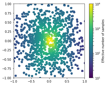
You might notice the information about the “effective number of samples” in the output. This is defined as 1 / max_events(weights); the smaller it is, the bigger the statistical fluctuations from too large weights. Let’s plot this over the parameter space:
cmin, cmax = 10., 10000.

cut = (y.flatten()==0)

fig = plt.figure(figsize=(5,4))

sc = plt.scatter(theta0[cut][:,0], theta0[cut][:,1], c=n_effective[cut],
                 s=30., cmap='viridis',
                 norm=matplotlib.colors.LogNorm(vmin=cmin, vmax=cmax),
                 marker='o')

cb = plt.colorbar(sc)
cb.set_label('Effective number of samples')

plt.xlim(-1.0,1.0)
plt.ylim(-1.0,1.0)
plt.tight_layout()
plt.show()
2. Plot cross section over parameter space#
This is not strictly necessary, but we can also plot the cross section as a function of parameter space:
thetas_benchmarks, xsecs_benchmarks, xsec_errors_benchmarks = sampler.cross_sections(
    theta=sampling.benchmarks(list(sampler.benchmarks.keys()))
)

thetas_morphing, xsecs_morphing, xsec_errors_morphing = sampler.cross_sections(
    theta=sampling.random_morphing_points(1000, [('gaussian', 0., 1.), ('gaussian', 0., 1.)])
)
20:37 madminer.sampling    INFO    Starting cross-section calculation
20:37 madminer.sampling    INFO    Starting cross-section calculation
cmin, cmax = 0., 2.5 * np.mean(xsecs_morphing)

fig = plt.figure(figsize=(5,4))

sc = plt.scatter(thetas_morphing[:,0], thetas_morphing[:,1], c=xsecs_morphing,
            s=40., cmap='viridis', vmin=cmin, vmax=cmax,
            marker='o')

plt.scatter(thetas_benchmarks[:,0], thetas_benchmarks[:,1], c=xsecs_benchmarks,
            s=200., cmap='viridis', vmin=cmin, vmax=cmax, lw=2., edgecolor='black',
            marker='s')

cb = plt.colorbar(sc)
cb.set_label('xsec [pb]')

plt.xlim(-3.,3.)
plt.ylim(-3.,3.)
plt.tight_layout()
plt.show()
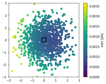
What you see here is a morphing algorithm in action. We only asked MadGraph to calculate event weights (differential cross sections, or basically squared matrix elements) at six fixed parameter points (shown here as squares with black edges). But with our knowledge about the structure of the process we can interpolate any observable to any parameter point without loss (except that statistical uncertainties might increase)!
3. Train likelihood ratio estimator#
It’s now time to build the neural network that estimates the likelihood ratio. The central object for this is the madminer.ml.ParameterizedRatioEstimator class. It defines functions that train, save, load, and evaluate the estimators.
In the initialization, the keywords n_hidden and activation define the architecture of the (fully connected) neural network:
estimator = ParameterizedRatioEstimator(
    n_hidden=(60,60),
    activation="tanh"
)
To train this model we will minimize the ALICES loss function described in “Likelihood-free inference with an improved cross-entropy estimator”. Many alternatives, including RASCAL, are described in “Constraining Effective Field Theories With Machine Learning” and “A Guide to Constraining Effective Field Theories With Machine Learning”. There is also SCANDAL introduced in “Mining gold from implicit models to improve likelihood-free inference”.
estimator.train(
    method='alices',
    theta='data/samples/theta0_train_ratio.npy',
    x='data/samples/x_train_ratio.npy',
    y='data/samples/y_train_ratio.npy',
    r_xz='data/samples/r_xz_train_ratio.npy',
    t_xz='data/samples/t_xz_train_ratio.npy',
    alpha=10,
    n_epochs=10,
    scale_parameters=True,
)

estimator.save('models/alices')
20:37 madminer.ml          INFO    Starting training
20:37 madminer.ml          INFO      Method:                 alices
20:37 madminer.ml          INFO      alpha:                  10
20:37 madminer.ml          INFO      Batch size:             128
20:37 madminer.ml          INFO      Optimizer:              amsgrad
20:37 madminer.ml          INFO      Epochs:                 10
20:37 madminer.ml          INFO      Learning rate:          0.001 initially, decaying to 0.0001
20:37 madminer.ml          INFO      Validation split:       0.25
20:37 madminer.ml          INFO      Early stopping:         True
20:37 madminer.ml          INFO      Scale inputs:           True
20:37 madminer.ml          INFO      Scale parameters:       True
20:37 madminer.ml          INFO      Shuffle labels          False
20:37 madminer.ml          INFO      Samples:                all
20:37 madminer.ml          INFO    Loading training data
20:37 madminer.utils.vario INFO      Loading data/samples/theta0_train_ratio.npy into RAM
20:37 madminer.utils.vario INFO      Loading data/samples/x_train_ratio.npy into RAM
20:37 madminer.utils.vario INFO      Loading data/samples/y_train_ratio.npy into RAM
20:37 madminer.utils.vario INFO      Loading data/samples/r_xz_train_ratio.npy into RAM
20:37 madminer.utils.vario INFO      Loading data/samples/t_xz_train_ratio.npy into RAM
20:37 madminer.ml          INFO    Found 500000 samples with 2 parameters and 3 observables
20:37 madminer.ml          INFO    Setting up input rescaling
20:37 madminer.ml          INFO    Rescaling parameters
20:37 madminer.ml          INFO    Setting up parameter rescaling
20:37 madminer.ml          INFO    Creating model
20:37 madminer.ml          INFO    Training model
20:37 madminer.utils.ml.tr INFO    Training on CPU with single precision
20:38 madminer.utils.ml.tr INFO      Epoch   1: train loss  1.03859 (improved_xe:  0.678, mse_score:  0.036)
20:38 madminer.utils.ml.tr INFO                 val. loss   0.96541 (improved_xe:  0.675, mse_score:  0.029)
20:39 madminer.utils.ml.tr INFO      Epoch   2: train loss  0.96694 (improved_xe:  0.675, mse_score:  0.029)
20:39 madminer.utils.ml.tr INFO                 val. loss   0.94460 (improved_xe:  0.675, mse_score:  0.027)
20:40 madminer.utils.ml.tr INFO      Epoch   3: train loss  0.95053 (improved_xe:  0.675, mse_score:  0.028)
20:40 madminer.utils.ml.tr INFO                 val. loss   0.93165 (improved_xe:  0.674, mse_score:  0.026)
20:41 madminer.utils.ml.tr INFO      Epoch   4: train loss  0.94048 (improved_xe:  0.675, mse_score:  0.027)
20:41 madminer.utils.ml.tr INFO                 val. loss   0.93224 (improved_xe:  0.675, mse_score:  0.026)
20:41 madminer.utils.ml.tr INFO      Epoch   5: train loss  0.93394 (improved_xe:  0.675, mse_score:  0.026)
20:41 madminer.utils.ml.tr INFO                 val. loss   0.92634 (improved_xe:  0.674, mse_score:  0.025)
20:42 madminer.utils.ml.tr INFO      Epoch   6: train loss  0.93002 (improved_xe:  0.674, mse_score:  0.026)
20:42 madminer.utils.ml.tr INFO                 val. loss   0.91939 (improved_xe:  0.674, mse_score:  0.025)
20:43 madminer.utils.ml.tr INFO      Epoch   7: train loss  0.92634 (improved_xe:  0.674, mse_score:  0.025)
20:43 madminer.utils.ml.tr INFO                 val. loss   0.91647 (improved_xe:  0.674, mse_score:  0.024)
20:44 madminer.utils.ml.tr INFO      Epoch   8: train loss  0.92436 (improved_xe:  0.674, mse_score:  0.025)
20:44 madminer.utils.ml.tr INFO                 val. loss   0.91579 (improved_xe:  0.674, mse_score:  0.024)
20:44 madminer.utils.ml.tr INFO      Epoch   9: train loss  0.92230 (improved_xe:  0.674, mse_score:  0.025)
20:44 madminer.utils.ml.tr INFO                 val. loss   0.91520 (improved_xe:  0.674, mse_score:  0.024)
20:45 madminer.utils.ml.tr INFO      Epoch  10: train loss  0.92073 (improved_xe:  0.674, mse_score:  0.025)
20:45 madminer.utils.ml.tr INFO                 val. loss   0.91580 (improved_xe:  0.674, mse_score:  0.024)
20:45 madminer.utils.ml.tr INFO    Early stopping after epoch 9, with loss  0.91520 compared to final loss  0.91580
20:45 madminer.utils.ml.tr INFO    Training time spend on:
20:45 madminer.utils.ml.tr INFO                      initialize model:   0.00h
20:45 madminer.utils.ml.tr INFO                                   ALL:   0.13h
20:45 madminer.utils.ml.tr INFO                            check data:   0.00h
20:45 madminer.utils.ml.tr INFO                          make dataset:   0.00h
20:45 madminer.utils.ml.tr INFO                       make dataloader:   0.00h
20:45 madminer.utils.ml.tr INFO                       setup optimizer:   0.00h
20:45 madminer.utils.ml.tr INFO                   initialize training:   0.00h
20:45 madminer.utils.ml.tr INFO                                set lr:   0.00h
20:45 madminer.utils.ml.tr INFO                   load training batch:   0.03h
20:45 madminer.utils.ml.tr INFO                        fwd: move data:   0.00h
20:45 madminer.utils.ml.tr INFO                   fwd: check for nans:   0.01h
20:45 madminer.utils.ml.tr INFO                    fwd: model.forward:   0.03h
20:45 madminer.utils.ml.tr INFO                 fwd: calculate losses:   0.01h
20:45 madminer.utils.ml.tr INFO                 training forward pass:   0.04h
20:45 madminer.utils.ml.tr INFO                   training sum losses:   0.00h
20:45 madminer.utils.ml.tr INFO                        opt: zero grad:   0.00h
20:45 madminer.utils.ml.tr INFO                         opt: backward:   0.02h
20:45 madminer.utils.ml.tr INFO                   opt: clip grad norm:   0.00h
20:45 madminer.utils.ml.tr INFO                             opt: step:   0.00h
20:45 madminer.utils.ml.tr INFO                        optimizer step:   0.03h
20:45 madminer.utils.ml.tr INFO                 load validation batch:   0.01h
20:45 madminer.utils.ml.tr INFO               validation forward pass:   0.01h
20:45 madminer.utils.ml.tr INFO                 validation sum losses:   0.00h
20:45 madminer.utils.ml.tr INFO                        early stopping:   0.00h
20:45 madminer.utils.ml.tr INFO                          report epoch:   0.00h
20:45 madminer.ml          INFO    Saving model to models/alices
Let’s for fun also train a model that only used pt_j1 as input observable, which can be specified using the option features when defining the ParameterizedRatioEstimator
estimator_pt = ParameterizedRatioEstimator(
    n_hidden=(40,40),
    activation="tanh",
    features=[0],
)

estimator_pt.train(
    method='alices',
    theta='data/samples/theta0_train_ratio.npy',
    x='data/samples/x_train_ratio.npy',
    y='data/samples/y_train_ratio.npy',
    r_xz='data/samples/r_xz_train_ratio.npy',
    t_xz='data/samples/t_xz_train_ratio.npy',
    alpha=8,
    n_epochs=10,
    scale_parameters=True,
)

estimator_pt.save('models/alices_pt')
20:45 madminer.ml          INFO    Starting training
20:45 madminer.ml          INFO      Method:                 alices
20:45 madminer.ml          INFO      alpha:                  8
20:45 madminer.ml          INFO      Batch size:             128
20:45 madminer.ml          INFO      Optimizer:              amsgrad
20:45 madminer.ml          INFO      Epochs:                 10
20:45 madminer.ml          INFO      Learning rate:          0.001 initially, decaying to 0.0001
20:45 madminer.ml          INFO      Validation split:       0.25
20:45 madminer.ml          INFO      Early stopping:         True
20:45 madminer.ml          INFO      Scale inputs:           True
20:45 madminer.ml          INFO      Scale parameters:       True
20:45 madminer.ml          INFO      Shuffle labels          False
20:45 madminer.ml          INFO      Samples:                all
20:45 madminer.ml          INFO    Loading training data
20:45 madminer.utils.vario INFO      Loading data/samples/theta0_train_ratio.npy into RAM
20:45 madminer.utils.vario INFO      Loading data/samples/x_train_ratio.npy into RAM
20:45 madminer.utils.vario INFO      Loading data/samples/y_train_ratio.npy into RAM
20:45 madminer.utils.vario INFO      Loading data/samples/r_xz_train_ratio.npy into RAM
20:45 madminer.utils.vario INFO      Loading data/samples/t_xz_train_ratio.npy into RAM
20:45 madminer.ml          INFO    Found 500000 samples with 2 parameters and 3 observables
20:45 madminer.ml          INFO    Setting up input rescaling
20:45 madminer.ml          INFO    Rescaling parameters
20:45 madminer.ml          INFO    Setting up parameter rescaling
20:45 madminer.ml          INFO    Only using 1 of 3 observables
20:45 madminer.ml          INFO    Creating model
20:45 madminer.ml          INFO    Training model
20:45 madminer.utils.ml.tr INFO    Training on CPU with single precision
20:46 madminer.utils.ml.tr INFO      Epoch   1: train loss  1.08569 (improved_xe:  0.684, mse_score:  0.050)
20:46 madminer.utils.ml.tr INFO                 val. loss   1.06532 (improved_xe:  0.682, mse_score:  0.048)
20:46 madminer.utils.ml.tr INFO      Epoch   2: train loss  1.05357 (improved_xe:  0.682, mse_score:  0.046)
20:46 madminer.utils.ml.tr INFO                 val. loss   1.06289 (improved_xe:  0.682, mse_score:  0.048)
20:47 madminer.utils.ml.tr INFO      Epoch   3: train loss  1.05015 (improved_xe:  0.682, mse_score:  0.046)
20:47 madminer.utils.ml.tr INFO                 val. loss   1.06356 (improved_xe:  0.682, mse_score:  0.048)
20:48 madminer.utils.ml.tr INFO      Epoch   4: train loss  1.04808 (improved_xe:  0.682, mse_score:  0.046)
20:48 madminer.utils.ml.tr INFO                 val. loss   1.05583 (improved_xe:  0.682, mse_score:  0.047)
20:49 madminer.utils.ml.tr INFO      Epoch   5: train loss  1.04594 (improved_xe:  0.682, mse_score:  0.046)
20:49 madminer.utils.ml.tr INFO                 val. loss   1.05662 (improved_xe:  0.682, mse_score:  0.047)
20:49 madminer.utils.ml.tr INFO      Epoch   6: train loss  1.04515 (improved_xe:  0.682, mse_score:  0.045)
20:49 madminer.utils.ml.tr INFO                 val. loss   1.05398 (improved_xe:  0.682, mse_score:  0.047)
20:50 madminer.utils.ml.tr INFO      Epoch   7: train loss  1.04437 (improved_xe:  0.682, mse_score:  0.045)
20:50 madminer.utils.ml.tr INFO                 val. loss   1.05249 (improved_xe:  0.682, mse_score:  0.046)
20:51 madminer.utils.ml.tr INFO      Epoch   8: train loss  1.04362 (improved_xe:  0.682, mse_score:  0.045)
20:51 madminer.utils.ml.tr INFO                 val. loss   1.05231 (improved_xe:  0.682, mse_score:  0.046)
20:52 madminer.utils.ml.tr INFO      Epoch   9: train loss  1.04301 (improved_xe:  0.682, mse_score:  0.045)
20:52 madminer.utils.ml.tr INFO                 val. loss   1.05363 (improved_xe:  0.682, mse_score:  0.046)
20:52 madminer.utils.ml.tr INFO      Epoch  10: train loss  1.04283 (improved_xe:  0.682, mse_score:  0.045)
20:52 madminer.utils.ml.tr INFO                 val. loss   1.05177 (improved_xe:  0.682, mse_score:  0.046)
20:52 madminer.utils.ml.tr INFO    Early stopping did not improve performance
20:52 madminer.utils.ml.tr INFO    Training time spend on:
20:52 madminer.utils.ml.tr INFO                      initialize model:   0.00h
20:52 madminer.utils.ml.tr INFO                                   ALL:   0.12h
20:52 madminer.utils.ml.tr INFO                            check data:   0.00h
20:52 madminer.utils.ml.tr INFO                          make dataset:   0.00h
20:52 madminer.utils.ml.tr INFO                       make dataloader:   0.00h
20:52 madminer.utils.ml.tr INFO                       setup optimizer:   0.00h
20:52 madminer.utils.ml.tr INFO                   initialize training:   0.00h
20:52 madminer.utils.ml.tr INFO                                set lr:   0.00h
20:52 madminer.utils.ml.tr INFO                   load training batch:   0.03h
20:52 madminer.utils.ml.tr INFO                        fwd: move data:   0.00h
20:52 madminer.utils.ml.tr INFO                   fwd: check for nans:   0.01h
20:52 madminer.utils.ml.tr INFO                    fwd: model.forward:   0.03h
20:52 madminer.utils.ml.tr INFO                 fwd: calculate losses:   0.01h
20:52 madminer.utils.ml.tr INFO                 training forward pass:   0.04h
20:52 madminer.utils.ml.tr INFO                   training sum losses:   0.00h
20:52 madminer.utils.ml.tr INFO                        opt: zero grad:   0.00h
20:52 madminer.utils.ml.tr INFO                         opt: backward:   0.02h
20:52 madminer.utils.ml.tr INFO                   opt: clip grad norm:   0.00h
20:52 madminer.utils.ml.tr INFO                             opt: step:   0.00h
20:52 madminer.utils.ml.tr INFO                        optimizer step:   0.03h
20:52 madminer.utils.ml.tr INFO                 load validation batch:   0.01h
20:52 madminer.utils.ml.tr INFO               validation forward pass:   0.01h
20:52 madminer.utils.ml.tr INFO                 validation sum losses:   0.00h
20:52 madminer.utils.ml.tr INFO                        early stopping:   0.00h
20:52 madminer.utils.ml.tr INFO                          report epoch:   0.00h
20:52 madminer.ml          INFO    Saving model to models/alices_pt
4. Evaluate likelihood ratio estimator#
estimator.evaluate_log_likelihood_ratio(theta,x) estimated the log likelihood ratio and the score for all combination between the given phase-space points x and parameters theta. That is, if given 100 events x and a grid of 25 theta points, it will return 25*100 estimates for the log likelihood ratio and 25*100 estimates for the score, both indexed by [i_theta,i_x].
theta_each = np.linspace(-1,1,25)
theta0, theta1 = np.meshgrid(theta_each, theta_each)
theta_grid = np.vstack((theta0.flatten(), theta1.flatten())).T
np.save('data/samples/theta_grid.npy', theta_grid)

theta_denom = np.array([[0.,0.]])
np.save('data/samples/theta_ref.npy', theta_denom)
estimator.load('models/alices')

log_r_hat, _ = estimator.evaluate_log_likelihood_ratio(
    theta='data/samples/theta_grid.npy',
    x='data/samples/x_test.npy',
    evaluate_score=False
)
20:52 madminer.ml          INFO    Loading model from models/alices
20:52 madminer.ml          INFO    Loading evaluation data
20:52 madminer.utils.vario INFO      Loading data/samples/x_test.npy into RAM
20:52 madminer.utils.vario INFO      Loading data/samples/theta_grid.npy into RAM
20:52 madminer.ml          INFO    Starting ratio evaluation for 625000 x-theta combinations
20:52 madminer.ml          INFO    Evaluation done
Let’s look at the result:
bin_size = theta_each[1] - theta_each[0]
edges = np.linspace(theta_each[0] - bin_size/2, theta_each[-1] + bin_size/2, len(theta_each)+1)

fig = plt.figure(figsize=(6,5))
ax = plt.gca()

expected_llr = np.mean(log_r_hat,axis=1)
best_fit = theta_grid[np.argmin(-2.*expected_llr)]

cmin, cmax = np.min(-2*expected_llr), np.max(-2*expected_llr)

pcm = ax.pcolormesh(edges, edges, -2. * expected_llr.reshape((25,25)),
                    norm=matplotlib.colors.Normalize(vmin=cmin, vmax=cmax),
                    cmap='viridis_r')
cbar = fig.colorbar(pcm, ax=ax, extend='both')

plt.scatter(best_fit[0], best_fit[1], s=80., color='black', marker='*')

plt.xlabel(r'$\theta_0$')
plt.ylabel(r'$\theta_1$')
cbar.set_label(r'$\mathbb{E}_x [ -2\, \log \,\hat{r}(x | \theta, \theta_{SM}) ]$')

plt.tight_layout()
plt.show()
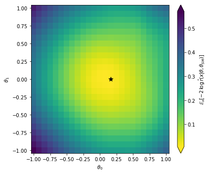
Note that in this tutorial our sample size was very small, and the network might not really have a chance to converge to the correct likelihood ratio function. So don’t worry if you find a minimum that is not at the right point (the SM, i.e. the origin in this plot). Feel free to dial up the event numbers in the run card as well as the training samples and see what happens then!